Chapter 10 Lecture Notes

This chapter consists of lecture notes from the class in Spring 2026.

10.1 January 27

Here is a summary of things to know from January 27.

The function lm creates a model of the data using only those rows which aren’t missing any values. This only applies to variables that are listed in the formula as the first argument of lm.
The formula for AIC is -2 log(likelhood) + 2k, where k is the number of parameters in the model. This means that AIC is explicitly balancing the fit of the model (the likelihood) with the number of parameters used. Lower values correspond to beter fits according to the AIC. AIC can only be used to compare two models that fit the exact same data.
When using MASS::stepAIC, there can often be errors which come up because when a variable us removed, the data set changes. For example, if y ~ x1 + x2 is the original model, and x2 is removed, and there is missing data in the variable x2, then when lm is run on y ~ x1, we are using a different data set. This causes an error in MASS::stepAIC.
We discussed several options for dealing with this.
1. Remove all rows from the data that contain any missing values before running stepAIC.
2. Every time stepAIC throws an error, remove that variable by hand from the original model and restart stepAIC from the beginning.
3. Remove variables from the model (if they have two many missing values).
4. Impute missing values. (We will learn how to do this later.)
We also discussed multiple \(R^2\) and adjusted \(R^2\). Let’s see how those values are computed. Multiple \(R^2\) is computed as \[ (\mathrm{var}(y) - \mathrm(var)(\eps))/\mathrm{var}(y) \] while adjusted \(R^2\) is computed the same, except we use the unbiased estimator for the variance of the residuals. Let’s look at an example:

set.seed(1)
x1 <- runif(30)
x2 <- runif(30)
y <- 1  + 2 * x1 + 3 * x2 + rnorm(30, 0, 1)
mod <- lm(y ~ x1 + x2)
summary(mod)

## 
## Call:
## lm(formula = y ~ x1 + x2)
## 
## Residuals:
##      Min       1Q   Median       3Q      Max 
## -1.38160 -0.52723 -0.02348  0.49973  1.45524 
## 
## Coefficients:
##             Estimate Std. Error t value Pr(>|t|)    
## (Intercept)   1.4601     0.4047   3.608  0.00124 ** 
## x1            2.4463     0.4822   5.073  2.5e-05 ***
## x2            1.9222     0.5779   3.326  0.00254 ** 
## ---
## Signif. codes:  0 '***' 0.001 '**' 0.01 '*' 0.05 '.' 0.1 ' ' 1
## 
## Residual standard error: 0.7664 on 27 degrees of freedom
## Multiple R-squared:  0.584,  Adjusted R-squared:  0.5532 
## F-statistic: 18.95 on 2 and 27 DF,  p-value: 7.207e-06

Let’s check that the formulas match the results from lm.

(var(y) - var(resid(mod)))/var(y)

## [1] 0.5840012

summary(mod)$r.sq

## [1] 0.5840012

(var(y) - sigma(mod)^2)/var(y)

## [1] 0.5531865

summary(mod)$adj

## [1] 0.5531865

The point is that our unbiased estimator for \(\sigma^2\) in the model depends on the number of parameters and is larger if we have more parameters. This means that, like AIC, the adjusted \(R^2\) is evaluating a trade-off between model fit and number of parameters.

Note: \(R^2\) is always between 0 and 1, while the adjusted \(R^2\) can be negative.

10.2 February 3

Here is a summary of things to know from February 3. The main goals were to understand interactions and multicollinearity of the predictors.

There are three types of interactions that we are going to be thinking about in this class. We will provide examples of each type of interaction in the context of exam scores as described by various predictors.

factor vs factor interaction Two factors interact when the effect of changing levels in one of the factors depends on which level the other factor has. As a made up example, suppose students are randomly assigned to study flashcards or to do practice problems in preparation for an exam. The students self-identify as having low prior knowledge or high prior knowledge before starting to study. Here is a chart giving mean scores on exam for the four groups of students.

knitr::kable(
  data.frame(
    `Prior Knowledge` = c("**Low**", "**High**"),
    Flashcards = c("**75**", "80"),
    `Practice Problems` = c("65", "**90**")
  ),
  align = "lcc",
  escape = FALSE,
  caption = "Effect of study method by prior knowledge"
)

Table 10.1: Effect of study method by prior knowledge
Prior.Knowledge	Flashcards	Practice.Problems
Low	75	65
High	80	90

As we can see, if the student has low prior knowledge, flashcards are more helpful, while if the student has high prior knowledge then practice problems are more helpful. That is an interaction between prior knowledge and study method, because the effect of changing from flaschards to practice problems depends on the prior knowledge of the student.

factor vs numeric interaction This is a very commonly studied interaction. In this case, the effect of changing a numerical predictor by one unit (the slope) depends on the level of a factor variable. As an example, consider scores on an exam as described by study time and prior knowledge. It is reasonable to expect that each hour of study will be more useful for someone with low prior knowledge, as illustrated in this table:

knitr::kable(
  data.frame(
    `Hours Studied` = c(2, 4, 6),
    `Low Prior Knowledge` = c(65, 75, 85),
    `High Prior Knowledge` = c(80, 84, 88)
  ),
  align = "rcc",
  caption = "Scores by hours studied and prior knowledge"
)

Table 10.2: Scores by hours studied and prior knowledge
Hours.Studied	Low.Prior.Knowledge	High.Prior.Knowledge
2	65	80
4	75	84
6	85	88

numeric vs numeric In this case, the effect of changing a numerical predictor by one unit (the slope) depends on the exact value of a different numeric variable. The model for this is \[ y ~ \beta_0 + \beta_1 x_1 + \beta_2 x_2 + \beta_3 x1 x_2 + \epsilon \] So that the change in slope of \(x_1\) depends in a very specific way on the value of the interaction variable \(x_2\). As an example, we model exam score by hours of sleep (before studying) and hours of studying. It is reasonable to expect that the more sleep you get, the more effective each hour of studying will be. Here is a sample chart of values:

knitr::kable(
  data.frame(
    `Hours Studied` = c(2, 4, 6),
    `Sleep = 2 hrs` = c(65, 66, 67),
    `Sleep = 4 hrs` = c(70, 72, 73),
    `Sleep = 6 hrs` = c(74, 80, 87),
    `Sleep = 8 hrs` = c(78, 86, 94)
  ),
  align = "rcccc",
  caption = "Scores by hours studied and hours of sleep"
)

Table 10.3: Scores by hours studied and hours of sleep
Hours.Studied	Sleep…2.hrs	Sleep…4.hrs	Sleep…6.hrs	Sleep…8.hrs
2	65	70	74	78
4	66	72	80	86
6	67	73	87	94

10.2.1 Simulating Data

R-Code Let’s look at how this works using R. We start by showing how to simulate data of each of the above types of interactions. There are two R functions that you might not be familiar with that we will use: case_when and pivot_wider. The function case_when is a way of encoding piecewise defined functions. For example, if you have \[ f(x) = \begin{cases} x + 1 &x < -1\\ 0 & -1 \le x \le 1\\ x - 1& x \ge 1 \end{cases} \] you can represent this by:

library(tidyverse)

## ── Attaching core tidyverse packages ──────────────────────── tidyverse 2.0.0 ──
## ✔ dplyr     1.1.4     ✔ readr     2.1.5
## ✔ forcats   1.0.0     ✔ stringr   1.5.1
## ✔ ggplot2   4.0.0     ✔ tibble    3.3.0
## ✔ lubridate 1.9.4     ✔ tidyr     1.3.1
## ✔ purrr     1.1.0     
## ── Conflicts ────────────────────────────────────────── tidyverse_conflicts() ──
## ✖ dplyr::filter() masks stats::filter()
## ✖ dplyr::lag()    masks stats::lag()
## ℹ Use the conflicted package (<http://conflicted.r-lib.org/>) to force all conflicts to become errors

f <- function(x) {
  case_when(
    x < -1 ~ x + 1,
    x >= -1 & x<= 1 ~ 0,
    x > 1 ~ x - 1
  )
}
curve(f(x), from = -3, to = 3)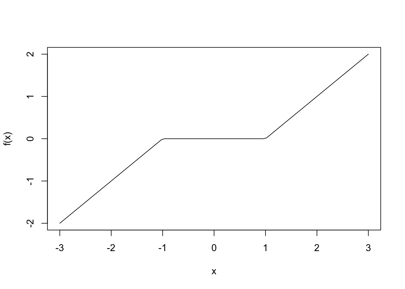

The function pivot_wider transforms a data set from long format to wide format. It is not essential to understand this function for this lecture, but so I will illustrate with an example. What if we want the babynames data set to have as each name as a row and the number of female and male babies as the data?

bb <- babynames::babynames
head(bb)

## # A tibble: 6 × 5
##    year sex   name          n   prop
##   <dbl> <chr> <chr>     <int>  <dbl>
## 1  1880 F     Mary       7065 0.0724
## 2  1880 F     Anna       2604 0.0267
## 3  1880 F     Emma       2003 0.0205
## 4  1880 F     Elizabeth  1939 0.0199
## 5  1880 F     Minnie     1746 0.0179
## 6  1880 F     Margaret   1578 0.0162

bb |> 
  filter(year == 2005) |> 
  select(name, n, sex) |> 
  pivot_wider(names_from = sex,
              values_from = n, 
              values_fill = 0) |> 
  arrange(desc(F + M))

## # A tibble: 30,153 × 3
##    name        F     M
##    <chr>   <int> <int>
##  1 Jacob      40 25830
##  2 Emily   23937    33
##  3 Michael    61 23812
##  4 Joshua     43 23248
##  5 Matthew    33 21467
##  6 Ethan      36 21309
##  7 Andrew     32 20727
##  8 Emma    20339    36
##  9 Daniel     50 20208
## 10 Madison 19566    80
## # ℹ 30,143 more rows

For factor vs factor interactions, cross-tables of means are often a good way to recognize the potential need for interactions; at least in the case you only have interaction between two variables.

#factor vs factor

x1 <- factor(c("low", "high"), levels = c("low", "high"))
x2 <- factor(c("flashcards", "practice_problems"))

dd <- data.frame(x1 = sample(x1, size = 30, replace = T),
                 x2 = sample(x2, size = 30, replace = T))
dd <- dd |> 
  mutate(y = case_when(
    x1 == "low" & x2 == "flashcards" ~ 75,
    x1 == "low" & x2 == "practice_problems" ~ 65,
    x1 == "high" & x2 == "flashcards" ~ 80,
    x1 == "high" & x2 == "practice_problems" ~ 90, #have to use vectorized & here
  ) + round(rnorm(30, 0, 10)))

dd |> 
  group_by(x1, x2) |> 
  summarize(mu = mean(y)) |> 
  pivot_wider(names_from = x2, values_from = mu)

## `summarise()` has grouped output by 'x1'. You can override using the `.groups`
## argument.

## # A tibble: 2 × 3
## # Groups:   x1 [2]
##   x1    flashcards practice_problems
##   <fct>      <dbl>             <dbl>
## 1 low         77.8              68.7
## 2 high        81.5              86.3

For factor vs numeric interactions, scatterplots with lines of best fit for each level of the factor are often a good way to recognize the potential need for interactions; at least in the case you only have interaction between two variables.

#factor vs numeric
x2 <- runif(30, 0, 10)
dd <- data.frame(x1 = sample(x1, size = 30, replace = T),
                 x2 = x2)

dd <- dd |> 
  mutate(y = case_when(
    x1 == "low" ~ 1 * x2,
    x1 == "high" ~ 2 * x2
  ) + rnorm(30, 0, 2))

dd |> 
  ggplot(aes(x = x2, y = y, color = x1)) + 
  geom_point() + 
  geom_smooth(method = "lm")

## `geom_smooth()` using formula = 'y ~ x'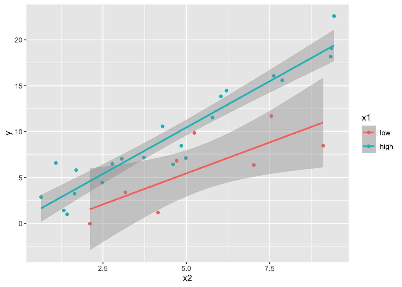

For numeric vs numeric, there are a few different ways of trying to recognize an interaction via exploratory vizualizations, but we will focus on plotting the line of best fit for several different intervals of one of the predictors. Let’s see how to simulate the data and to vizualize.

#numeric vs numeric
n <- 400 #bigger so that we can see things clearly; need plenty of data to have clear results
sleep <- runif(n, 2, 9)
study <- runif(n, 1, 6)

dd <- data.frame(sleepc = sleep - mean(sleep),
                 studyc = study - mean(study))

dd <- dd |> 
    mutate(score = round(78 + 4.0 * studyc + 3.0 * sleepc + 1.4 * studyc * sleepc + rnorm(n, 0, 4.5), 1))

dd |> 
  mutate(sleepint = cut(sleepc, 3)) |> #this creates 3 roughly equal groups in the sleep score
  ggplot(aes(x = studyc, y = score, color = sleepint)) + 
  geom_point() + 
  geom_smooth(method = "lm")

## `geom_smooth()` using formula = 'y ~ x'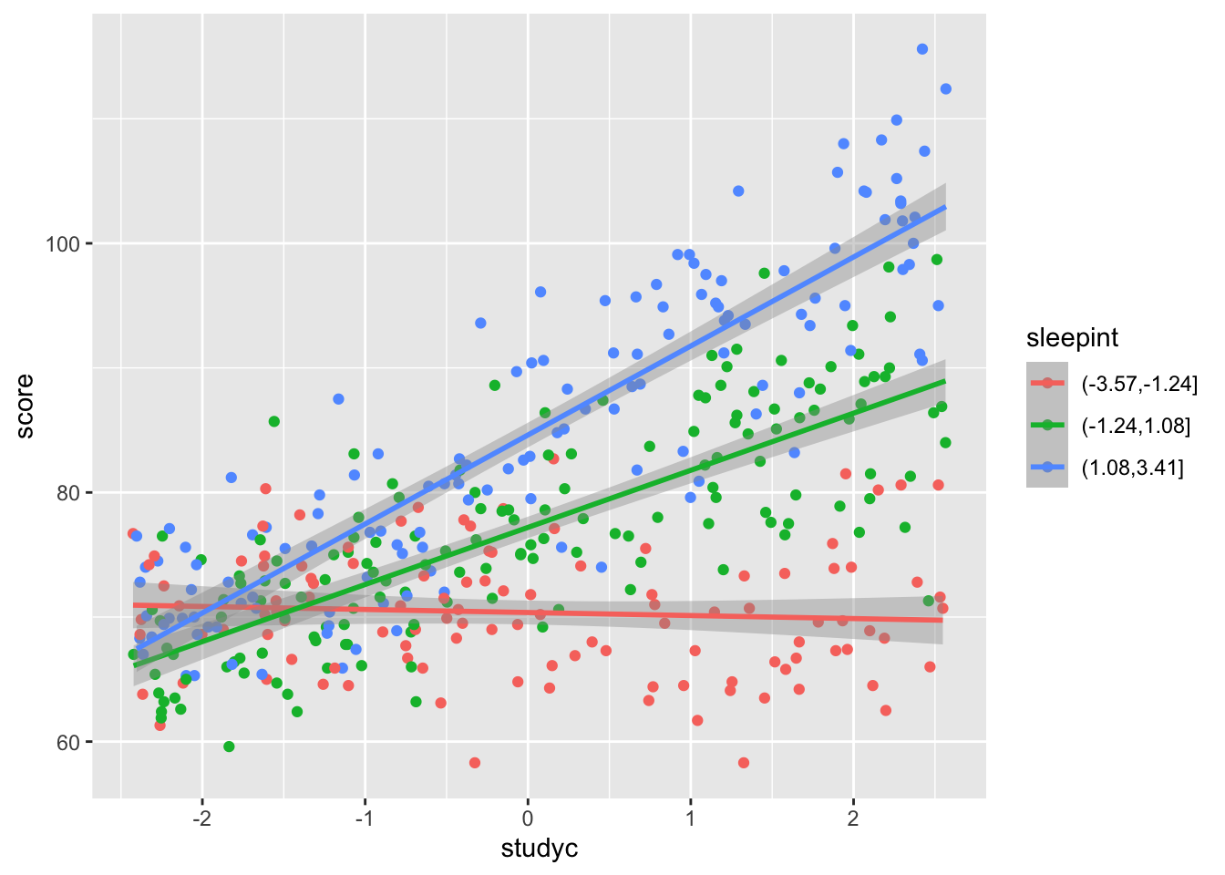

#compare what happens when we take the coefficient to be near 0

10.2.2 Building Models

We will build models on our simulated data above as well as on real data sets to see what is going on.

10.2.2.1 factor vs factor:

x1 <- factor(c("low", "high"), levels = c("low", "high"))
x2 <- factor(c("flashcards", "practice_problems"))

dd <- data.frame(x1 = sample(x1, size = 30, replace = T),
                 x2 = sample(x2, size = 30, replace = T))
dd <- dd |> 
  mutate(y = case_when(
    x1 == "low" & x2 == "flashcards" ~ 75,
    x1 == "low" & x2 == "practice_problems" ~ 65,
    x1 == "high" & x2 == "flashcards" ~ 80,
    x1 == "high" & x2 == "practice_problems" ~ 90, #have to use vectorized & here
  ) + round(rnorm(30, 0, 10)))

mod <- lm(y ~ x1 * x2, data = dd)
summary(mod) #interpret this into predictions/expected values for the combinations of levels!

## 
## Call:
## lm(formula = y ~ x1 * x2, data = dd)
## 
## Residuals:
##      Min       1Q   Median       3Q      Max 
## -17.3333  -7.1333   0.1111   7.4778  15.6667 
## 
## Coefficients:
##                            Estimate Std. Error t value Pr(>|t|)    
## (Intercept)                  73.000      3.010  24.254  < 2e-16 ***
## x1high                        4.889      4.373   1.118 0.273829    
## x2practice_problems         -10.600      5.213  -2.033 0.052350 .  
## x1high:x2practice_problems   27.044      7.235   3.738 0.000922 ***
## ---
## Signif. codes:  0 '***' 0.001 '**' 0.01 '*' 0.05 '.' 0.1 ' ' 1
## 
## Residual standard error: 9.518 on 26 degrees of freedom
## Multiple R-squared:  0.5631, Adjusted R-squared:  0.5127 
## F-statistic: 11.17 on 3 and 26 DF,  p-value: 6.819e-05

Consider the penguins data set. Is there evidence of an interaction between species and sex when predicting body_mass?

penguins |> 
  filter(!is.na(sex)) |> 
  group_by(species, sex) |> 
  summarize(mu = mean(body_mass)) |> 
  pivot_wider(names_from = sex, values_from = mu)

## `summarise()` has grouped output by 'species'. You can override using the
## `.groups` argument.

## # A tibble: 3 × 3
## # Groups:   species [3]
##   species   female  male
##   <fct>      <dbl> <dbl>
## 1 Adelie     3369. 4043.
## 2 Chinstrap  3527. 3939.
## 3 Gentoo     4680. 5485.

mod <- lm(body_mass ~ species * sex, data = penguins)
summary(mod)

## 
## Call:
## lm(formula = body_mass ~ species * sex, data = penguins)
## 
## Residuals:
##     Min      1Q  Median      3Q     Max 
## -827.21 -213.97   11.03  206.51  861.03 
## 
## Coefficients:
##                          Estimate Std. Error t value Pr(>|t|)    
## (Intercept)               3368.84      36.21  93.030  < 2e-16 ***
## speciesChinstrap           158.37      64.24   2.465  0.01420 *  
## speciesGentoo             1310.91      54.42  24.088  < 2e-16 ***
## sexmale                    674.66      51.21  13.174  < 2e-16 ***
## speciesChinstrap:sexmale  -262.89      90.85  -2.894  0.00406 ** 
## speciesGentoo:sexmale      130.44      76.44   1.706  0.08886 .  
## ---
## Signif. codes:  0 '***' 0.001 '**' 0.01 '*' 0.05 '.' 0.1 ' ' 1
## 
## Residual standard error: 309.4 on 327 degrees of freedom
##   (11 observations deleted due to missingness)
## Multiple R-squared:  0.8546, Adjusted R-squared:  0.8524 
## F-statistic: 384.3 on 5 and 327 DF,  p-value: < 2.2e-16

What is the predicted/expected body mass of a male chinstrap penguin? This would make a good exam problem; I give you the ouptut and you interpret.

10.2.2.2 factor vs numeric

x2 <- runif(30, 0, 10)
dd <- data.frame(x1 = sample(x1, size = 30, replace = T),
                 x2 = x2)

dd <- dd |> 
  mutate(y = case_when(
    x1 == "low" ~ 1 * x2,
    x1 == "high" ~ 2 * x2
  ) + rnorm(30, 0, 2))
mod <- lm(y ~ x1 * x2, data = dd)
summary(mod)

## 
## Call:
## lm(formula = y ~ x1 * x2, data = dd)
## 
## Residuals:
##     Min      1Q  Median      3Q     Max 
## -3.8866 -0.9466 -0.0584  1.1618  3.6873 
## 
## Coefficients:
##             Estimate Std. Error t value Pr(>|t|)    
## (Intercept)   1.2163     1.3182   0.923  0.36466    
## x1high       -1.6386     1.7188  -0.953  0.34917    
## x2            0.8376     0.1976   4.239  0.00025 ***
## x1high:x2     1.2678     0.2726   4.650 8.46e-05 ***
## ---
## Signif. codes:  0 '***' 0.001 '**' 0.01 '*' 0.05 '.' 0.1 ' ' 1
## 
## Residual standard error: 2.029 on 26 degrees of freedom
## Multiple R-squared:  0.8715, Adjusted R-squared:  0.8566 
## F-statistic: 58.76 on 3 and 26 DF,  p-value: 1.026e-11

penguins |>
  ggplot(aes(x = bill_len, y = body_mass, color = species)) + 
  geom_point() + 
  geom_smooth(method = "lm")

## `geom_smooth()` using formula = 'y ~ x'

## Warning: Removed 2 rows containing non-finite outside the scale range
## (`stat_smooth()`).

## Warning: Removed 2 rows containing missing values or values outside the scale range
## (`geom_point()`).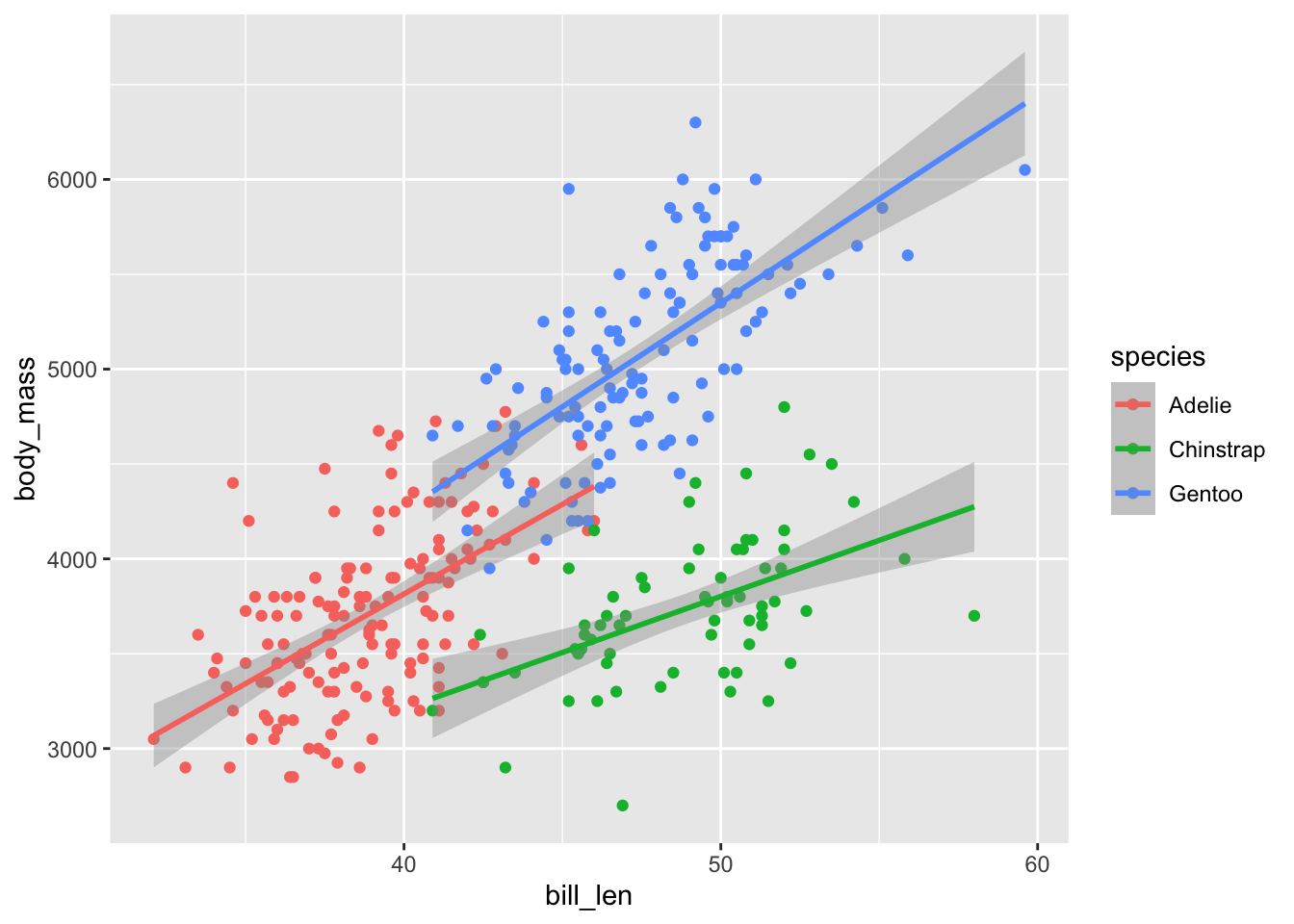

mod <- lm(body_mass ~ bill_len * species, data = penguins)
summary(mod) #barely significant, but significant

## 
## Call:
## lm(formula = body_mass ~ bill_len * species, data = penguins)
## 
## Residuals:
##     Min      1Q  Median      3Q     Max 
## -918.76 -245.89   -8.65  238.44 1126.27 
## 
## Coefficients:
##                           Estimate Std. Error t value Pr(>|t|)    
## (Intercept)                  34.88     443.18   0.079    0.937    
## bill_len                     94.50      11.40   8.291 2.73e-15 ***
## speciesChinstrap            811.26     799.81   1.014    0.311    
## speciesGentoo              -158.71     683.19  -0.232    0.816    
## bill_len:speciesChinstrap   -35.38      17.75  -1.994    0.047 *  
## bill_len:speciesGentoo       14.96      15.79   0.948    0.344    
## ---
## Signif. codes:  0 '***' 0.001 '**' 0.01 '*' 0.05 '.' 0.1 ' ' 1
## 
## Residual standard error: 371.8 on 336 degrees of freedom
##   (2 observations deleted due to missingness)
## Multiple R-squared:  0.7882, Adjusted R-squared:  0.7851 
## F-statistic: 250.1 on 5 and 336 DF,  p-value: < 2.2e-16

10.2.2.3 numeric vs numeric

n <- 400 #bigger so that we can see things clearly; need plenty of data to have clear results
sleep <- runif(n, 2, 9)
study <- runif(n, 1, 6)

dd <- data.frame(sleepc = sleep - mean(sleep),
                 studyc = study - mean(study))

dd <- dd |> 
    mutate(score = round(78 + 4.0 * studyc + 3.0 * sleepc + 1.4 * studyc * sleepc + rnorm(n, 0, 4.5), 1))
mod <- lm(score ~ sleepc * studyc, data = dd)
summary(mod)

## 
## Call:
## lm(formula = score ~ sleepc * studyc, data = dd)
## 
## Residuals:
##      Min       1Q   Median       3Q      Max 
## -13.2418  -2.7766   0.0401   3.4414  14.3340 
## 
## Coefficients:
##               Estimate Std. Error t value Pr(>|t|)    
## (Intercept)    77.9174     0.2431  320.46   <2e-16 ***
## sleepc          3.0431     0.1201   25.34   <2e-16 ***
## studyc          3.9047     0.1696   23.02   <2e-16 ***
## sleepc:studyc   1.4204     0.0852   16.67   <2e-16 ***
## ---
## Signif. codes:  0 '***' 0.001 '**' 0.01 '*' 0.05 '.' 0.1 ' ' 1
## 
## Residual standard error: 4.851 on 396 degrees of freedom
## Multiple R-squared:  0.7912, Adjusted R-squared:  0.7896 
## F-statistic: 500.1 on 3 and 396 DF,  p-value: < 2.2e-16

penguins |> 
  mutate(bill_len = cut(bill_len, 4)) |> 
  ggplot(aes(x = bill_dep, y = body_mass, color = bill_len)) + 
  geom_point() +
  geom_smooth(method = "lm") #oof, this is terrible; we should not build a model based on this. why?

## `geom_smooth()` using formula = 'y ~ x'

## Warning: Removed 2 rows containing non-finite outside the scale range
## (`stat_smooth()`).

## Warning: Removed 2 rows containing missing values or values outside the scale range
## (`geom_point()`).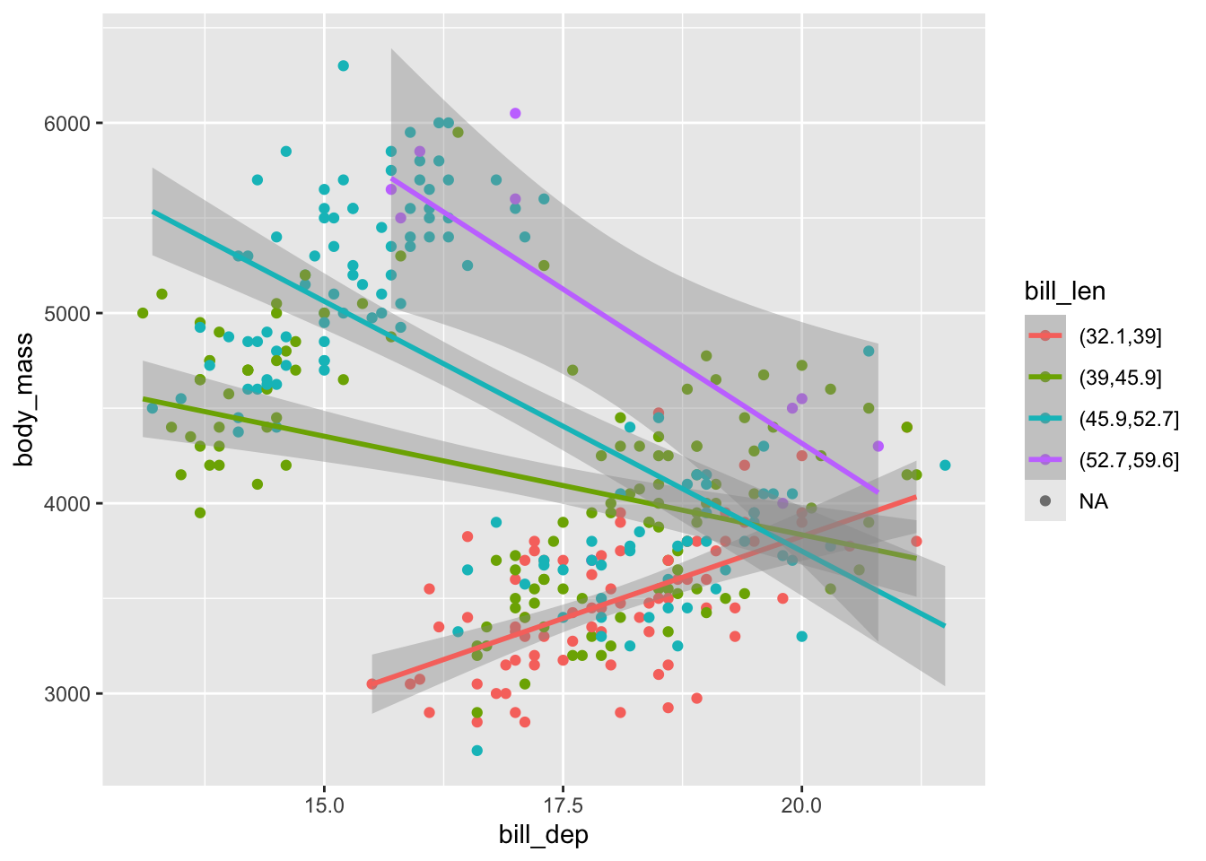

10.3 February 5

Here is a summary of things to know from February 5. We focused on multicollinearity of the predictors in a regression model and understanding one-way and two-way ANOVA models. But first, a quick “review” of how to augment a data fram a model.

10.3.1 Using `broom::augment`

The easiest way to add fitted values and residuals to a data frame is to use the broom::augment function. Here is an example using the penguins data set.

library(broom) #part of the tidyverse, but not the tidyverse package
mod <- lm(body_mass ~ bill_len + bill_dep + flipper_len, data = penguins)
augmented_data <- broom::augment(mod) #this is in the broom package
head(augmented_data)

## # A tibble: 6 × 11
##   .rownames body_mass bill_len bill_dep flipper_len .fitted .resid    .hat
##   <chr>         <int>    <dbl>    <dbl>       <int>   <dbl>  <dbl>   <dbl>
## 1 1              3750     39.1     18.7         181   3212.  538.  0.00883
## 2 2              3800     39.5     17.4         186   3439.  361.  0.00731
## 3 3              3250     40.3     18           195   3906. -656.  0.00460
## 4 5              3450     36.7     19.3         193   3817. -367.  0.0133 
## 5 6              3650     39.3     20.6         190   3703.  -53.0 0.0143 
## 6 7              3625     38.9     17.8         181   3193.  432.  0.00999
## # ℹ 3 more variables: .sigma <dbl>, .cooksd <dbl>, .std.resid <dbl>

Let’s look at each of the new variables.

.fitted are the fitted values from the model.
.resid are the residuals from the model.
.hat are the leverages from the model. These measure how far away each observation is from the center of the data in terms of the predictor variables.
.sigma are the standard deviations of the residuals after removing each observation one at a time.
.cooksd are Cook’s distances, which measure how much influence each observation has; that is how much the fitted values would change if we removed that observation from the data set and refit the model.
.std.resid are the standardized residuals, which are the residuals divided by their standard deviation. These are useful for finding outliers in the response variable.

Let’s look at an example or two to see what is going on.

n <- 10
x <- c(runif(n - 1), 10) 
y <- x + 2 + rnorm(n, 0, 1)
mod <- lm(y ~ x)
augmented_data <- broom::augment(mod)
augmented_data

## # A tibble: 10 × 8
##         y       x .fitted .resid  .hat .sigma   .cooksd .std.resid
##     <dbl>   <dbl>   <dbl>  <dbl> <dbl>  <dbl>     <dbl>      <dbl>
##  1  1.54   0.284     1.94 -0.401 0.118   1.60   0.00541     -0.284
##  2  3.20   0.748     2.42  0.780 0.107   1.58   0.0180       0.548
##  3  1.41   0.613     2.28 -0.870 0.110   1.57   0.0231      -0.612
##  4  3.11   0.513     2.18  0.937 0.112   1.57   0.0275       0.660
##  5  0.306  0.874     2.55 -2.25  0.105   1.34   0.146       -1.58 
##  6  4.30   0.0133    1.66  2.65  0.128   1.20   0.259        1.88 
##  7  1.84   0.555     2.22 -0.381 0.111   1.60   0.00449     -0.268
##  8  3.58   0.924     2.60  0.971 0.104   1.56   0.0270       0.681
##  9  0.596  0.535     2.20 -1.60  0.112   1.48   0.0803      -1.13 
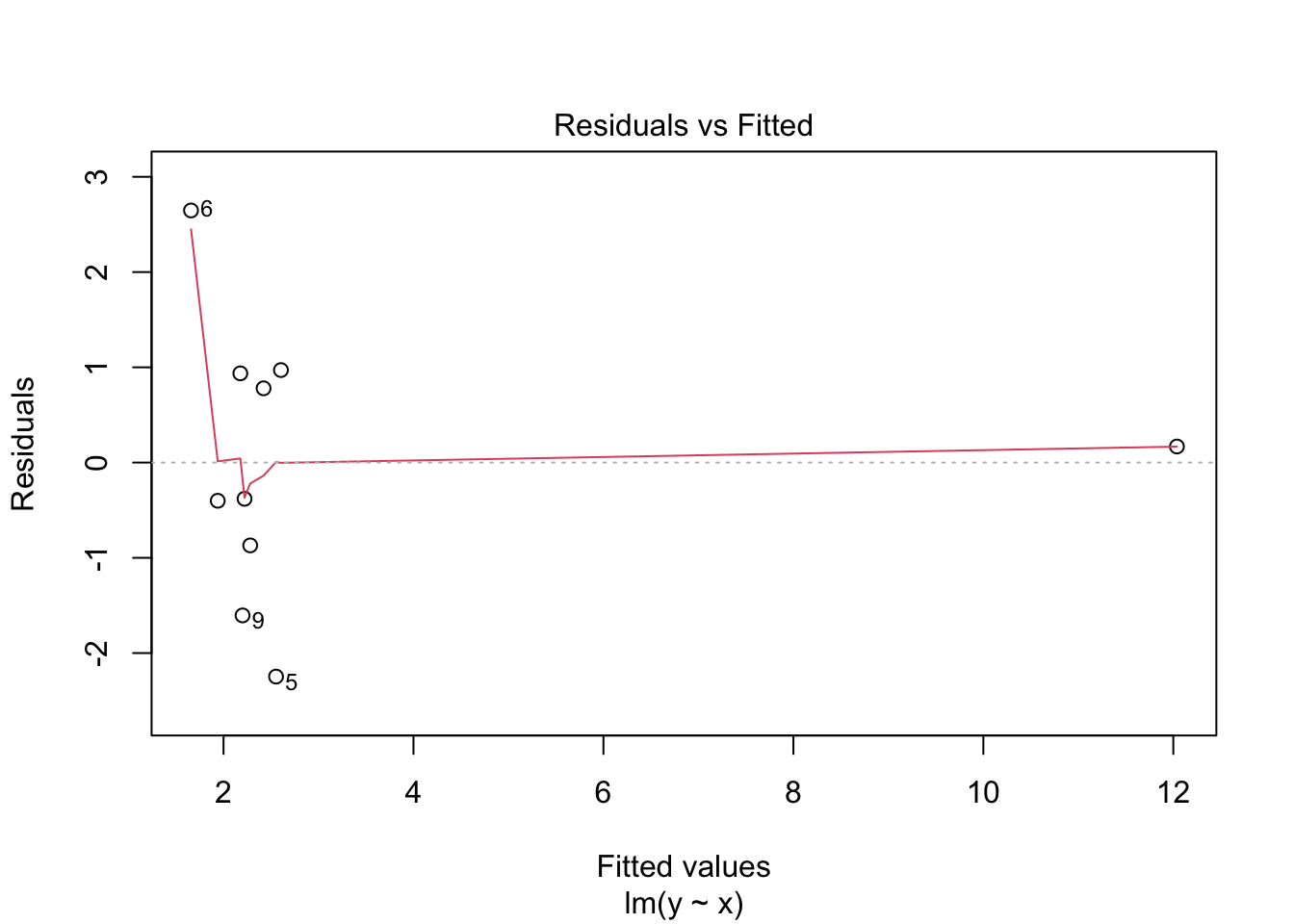
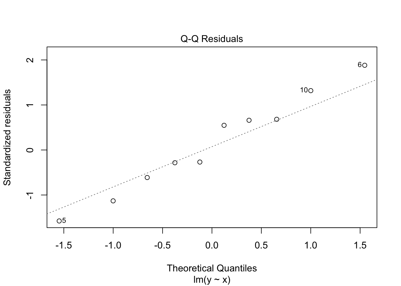
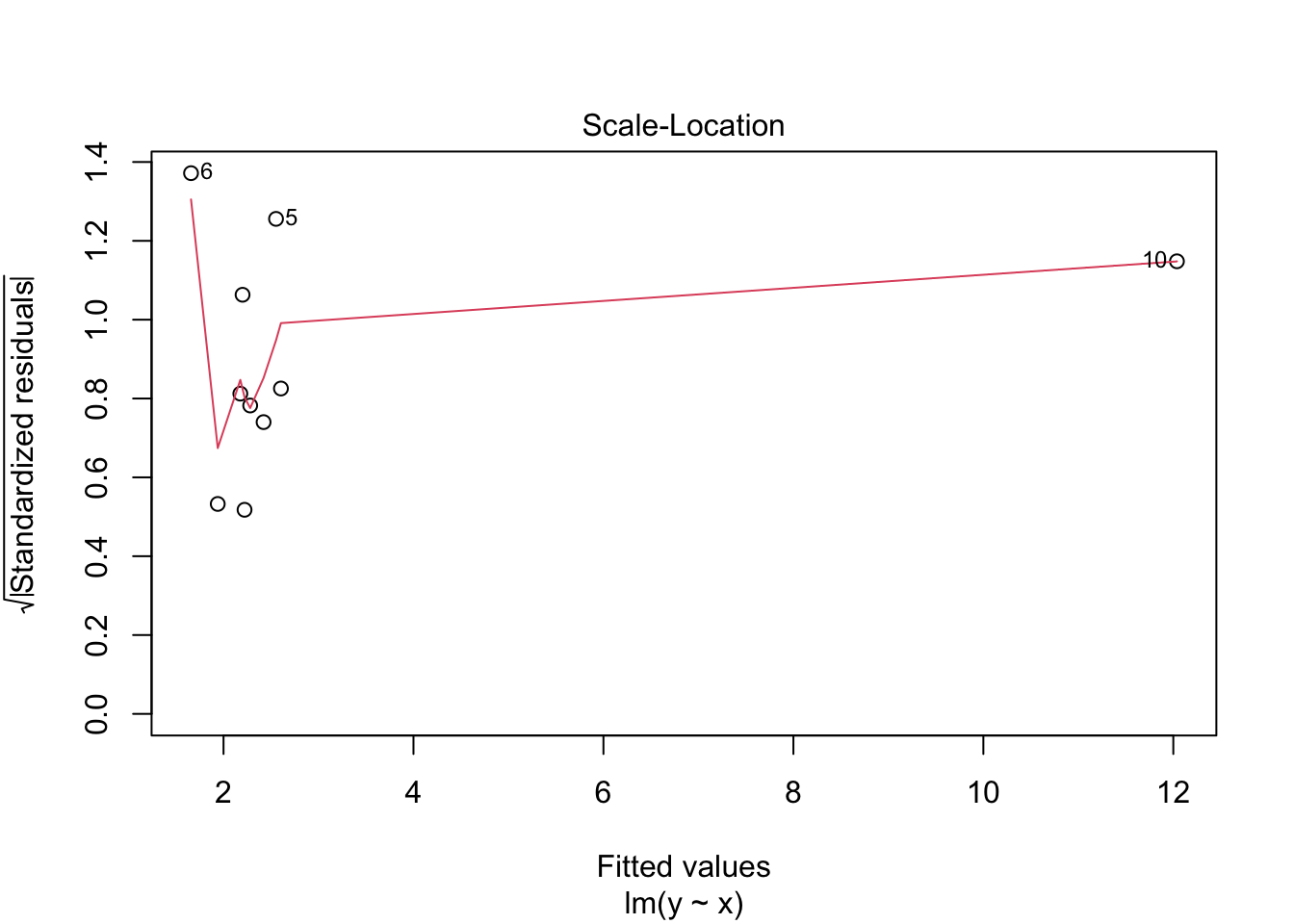
## 10 12.2   10        12.0   0.169 0.993   1.42 120.           1.32

Note that both the leverage and Cook’s distance are large for the last observation, which is an outlier in the predictor variable.

plot(mod) #this also shows the same thing

## Warning in sqrt(crit * p * (1 - hh)/hh): NaNs produced
## Warning in sqrt(crit * p * (1 - hh)/hh): NaNs produced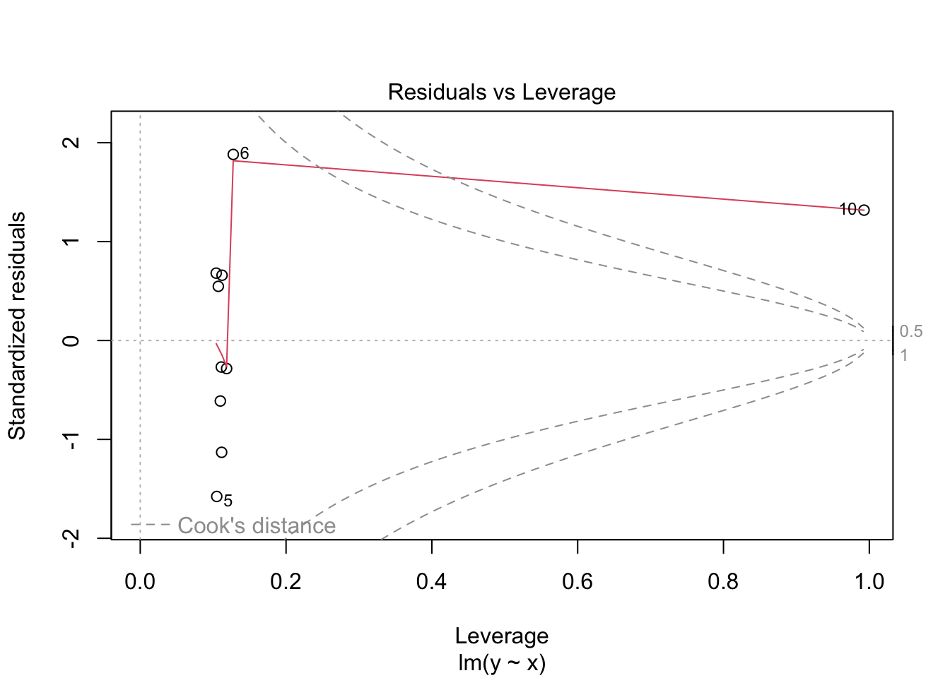

n <- 10
x <- c(runif(n)) 
y <- x + 2 + rnorm(n, 0, 1)
y[which.max(x)] <- 20 #make the last one an outlier in y  
mod <- lm(y ~ x)
augmented_data <- broom::augment(mod)
augmented_data

## # A tibble: 10 × 8
##        y      x .fitted  .resid  .hat .sigma    .cooksd .std.resid
##    <dbl>  <dbl>   <dbl>   <dbl> <dbl>  <dbl>      <dbl>      <dbl>
##  1 20    0.983    9.87  10.1    0.433  0.812 2.97          2.79   
##  2  1.61 0.0282  -0.728  2.34   0.311  5.03  0.0771        0.585  
##  3  2.31 0.862    8.54  -6.23   0.299  4.31  0.509        -1.54   
##  4  1.55 0.177    0.930  0.623  0.188  5.14  0.00239       0.144  
##  5  1.52 0.660    6.29  -4.77   0.151  4.76  0.103        -1.08   
##  6  2.85 0.456    4.02  -1.17   0.100  5.12  0.00363      -0.256  
##  7  2.49 0.316    2.47   0.0227 0.122  5.15  0.00000176    0.00504
##  8  3.36 0.167    0.816  2.54   0.195  5.03  0.0421        0.589  
##  9  2.87 0.430    3.73  -0.862  0.101  5.13  0.00199      -0.189  
## 10  1.17 0.435    3.79  -2.63   0.100  5.04  0.0184       -0.575

Note that the standardized residual is large for the largest observation, which is an outlier in the response variable. In this case, .sigma is also much smaller for that observation, because removing it makes the residuals much smaller. The Cook’s distance is also large, because removing that observation would change the fitted values a lot. However, the leverage is not large, because that observation is not far away from the center of the data in terms of the predictor variable.

10.3.2 Multicollinearity

Multicollinearity occurs when two or more predictor variables are highly correlated with each other. This can cause problems in regression models, because it can make it difficult to determine the individual effect of each predictor on the response variable. It generally does not negatively affect the overall predictive power of the model, but it can make the coefficients unstable and difficult to interpret.

To detect multicollinearity, we can use the Variance Inflation Factor (VIF). A VIF value greater than 5 or 10 is often considered indicative of multicollinearity. Variance Inflation Factor can be computed using the car package in R.car::vif computes the variance inflation factor by regressing each predictor on all the other predictors and computing the \(R^2\) value for that regression. The VIF is then computed as \[ VIF_j = \frac{1}{1 - R_j^2} \]

Let’s look at a simulated example with multicollinearity.

set.seed(1)
n <- 100
x1 <- rnorm(n)
x2 <- 0.9 * x1 + rnorm(n, 0, .1) #highly correlated with x
x3 <- rnorm(n) #not correlated with x1
y <- 3 + 2 * x1 + 0.5 * x2 + 1 * x3 + rnorm(n, 0, 1)
mod <- lm(y ~ x1 + x2 + x3)
summary(mod)

## 
## Call:
## lm(formula = y ~ x1 + x2 + x3)
## 
## Residuals:
##      Min       1Q   Median       3Q      Max 
## -2.58201 -0.52738  0.00281  0.65058  1.82364 
## 
## Coefficients:
##             Estimate Std. Error t value Pr(>|t|)    
## (Intercept)  3.05273    0.10065  30.331   <2e-16 ***
## x1           2.43652    0.95019   2.564   0.0119 *  
## x2          -0.04942    1.04845  -0.047   0.9625    
## x3           1.10462    0.09712  11.374   <2e-16 ***
## ---
## Signif. codes:  0 '***' 0.001 '**' 0.01 '*' 0.05 '.' 0.1 ' ' 1
## 
## Residual standard error: 0.998 on 96 degrees of freedom
## Multiple R-squared:  0.8616, Adjusted R-squared:  0.8573 
## F-statistic: 199.2 on 3 and 96 DF,  p-value: < 2.2e-16

car::vif(mod) #high VIF for x1 and x2

##        x1        x2        x3 
## 72.395291 72.382006  1.002798

Note the large standard errors for the coefficients of x1 and x2, as well as the high VIF values.

One would expect that if we ran this model many times and looked at the coefficients for x1 and x2, they would vary widely from one model to the next, because of the multicollinearity. However, the sum of the two coefficients should be more stable, because that is the combined effect of x1 and x2. Let’s check this out by simulating the model 1000 times and looking at the distribution of the coefficients.

For this simulation, we introduce purrr::map_df, which is a function that applies a function to each element of a list and returns the results as a data frame. Here, we use it to run the simulation 1000 times and collect the results.

simdata <- purrr::map_df(1:1000, function(x) {
  x1 <- rnorm(n)
  x2 <- 0.9 * x1 + rnorm(n, 0, .1) #highly correlated with x
  x3 <- rnorm(n) #not correlated with x1
  y <- 3 + 2 * x1 + 0.5 * x2 + 1 * x3 + rnorm(n, 0, 1)
  mod <- lm(y ~ x1 + x2 + x3)
  broom::tidy(mod) |>  #returns a data frame with the coefficients
    mutate(trial = x)
})

simdata |> 
  filter(term %in% c("x1", "x2")) |> 
  ggplot(aes(x = estimate, fill = term)) + 
  geom_density(alpha = 0.5) + 
  labs(title = "Distribution of Coefficients for x1 and x2",
       x = "Coefficient Estimate",
       y = "Density")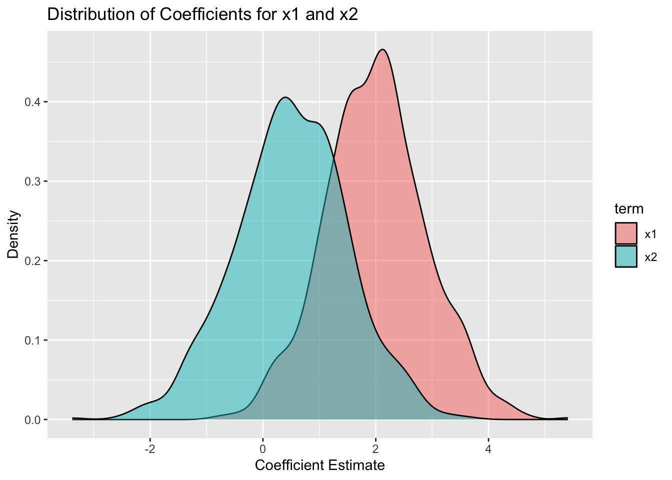

#let's compare that to the distribution of the sum of the coefficients

simdata |> 
  filter(term %in% c("x1", "x2")) |> 
  group_by(trial) |> 
  summarize(sum_estimate = sum(estimate)) |> 
  ggplot(aes(x = sum_estimate)) + 
  geom_density(fill = "blue", alpha = 0.5) + 
  labs(title = "Distribution of Sum of Coefficients for x1 and x2",
       x = "Sum of Coefficient Estimates",
       y = "Density") + 
  scale_x_continuous(limits = c(-3, 5))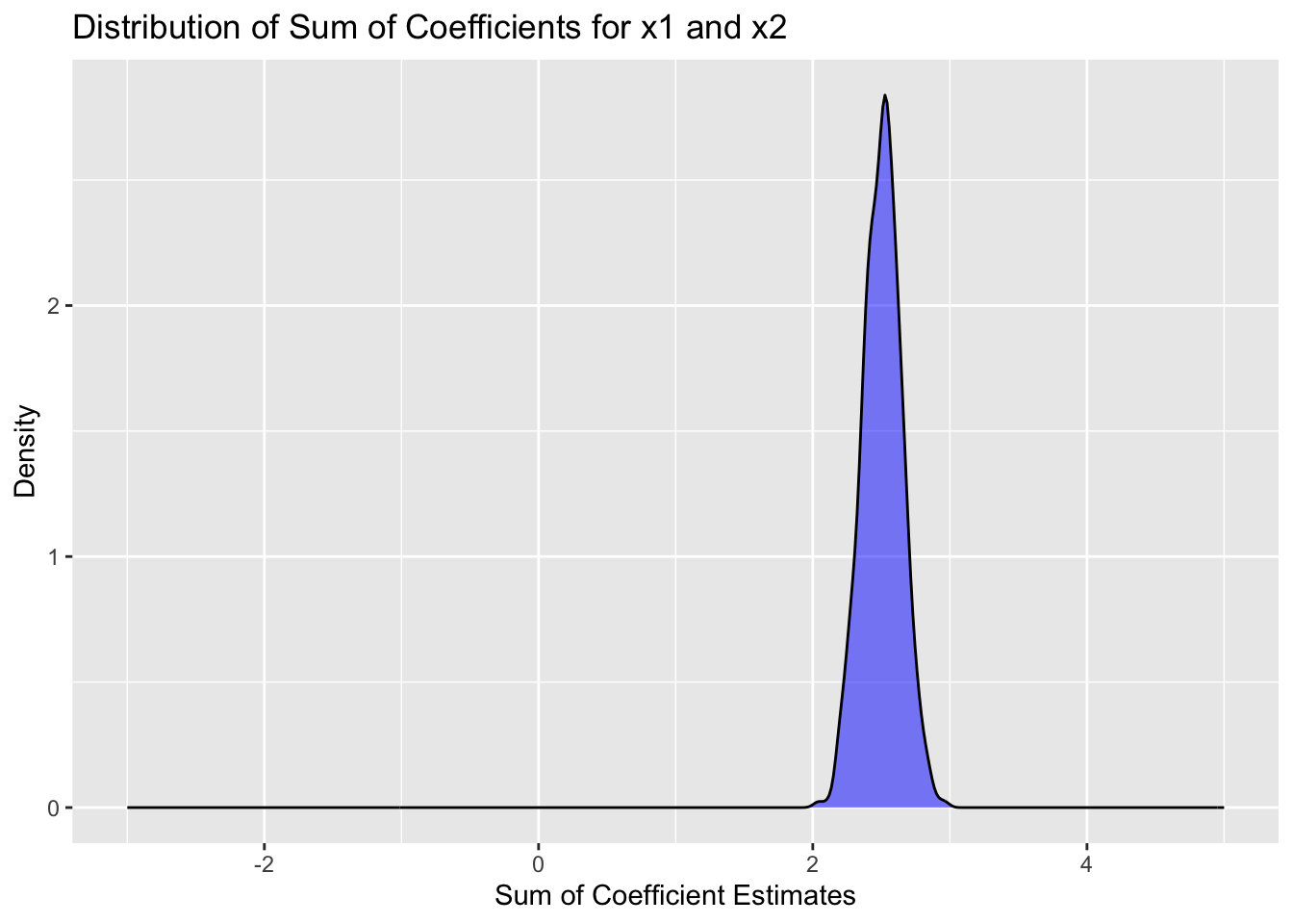

We see that the “correct” interpretation is that the sum of the coefficients for x1 and x2 is about 2.5, which is what we would expect from the data generating process. However, the individual coefficients vary widely from one simulation to the next, and would be hard to interpret.

What should you do if you discover multicollinearity in your data? Here are some options:

Do nothing. If your goal is prediction only, then multicollinearity may not be a problem. If interpretation is still your goal, you can try to interpret the highly correlated variables jointly, rather than individually.
Remove one or more of the correlated predictors from the model. Often you will choose to keep the variable that is either cheaper to measure, more fundamental theoretically, or more interpretable.
Combine the correlated predictors into a single predictor (e.g., by taking their average or sum). This is often used when you have domain knowledge of the predictors. For example, height and weight could be combined into a body mass index (BMI) variable. Or section scores of the ACT could be combined into a total score.
Use regularization techniques (e.g., ridge regression or lasso) that can handle multicollinearity. (We have not yet covered this material.)

As a summary, multicollinearity does not break your model. It is not an assumption of OLS that the predictors are uncorrelated. However, it can make interpretation of the coefficients difficult, and can lead to large standard errors for the coefficients.

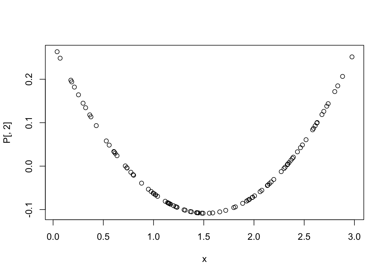
As another example, let’s look at so-called polynomial regression, where we include powers of a predictor variable in the model. This can also lead to multicollinearity.

set.seed(1)
n <- 100
x <- runif(n, 0, 3)
y <- 2 + 1.5 * x - 0.5 * x^2 + 0.3 * x^3 + rnorm(n, 0, 1)
mod <- lm(y ~ x + I(x^2) + I(x^3)) #using raw = TRUE to get x, x^2, x^3
summary(mod)

## 
## Call:
## lm(formula = y ~ x + I(x^2) + I(x^3))
## 
## Residuals:
##      Min       1Q   Median       3Q      Max 
## -1.85466 -0.59246 -0.09722  0.54144  2.48360 
## 
## Coefficients:
##             Estimate Std. Error t value Pr(>|t|)    
## (Intercept)   1.6348     0.4645   3.519 0.000664 ***
## x             2.2065     1.2415   1.777 0.078695 .  
## I(x^2)       -0.9631     0.9473  -1.017 0.311866    
## I(x^3)        0.3993     0.2099   1.902 0.060190 .  
## ---
## Signif. codes:  0 '***' 0.001 '**' 0.01 '*' 0.05 '.' 0.1 ' ' 1
## 
## Residual standard error: 0.9496 on 96 degrees of freedom
## Multiple R-squared:  0.8326, Adjusted R-squared:  0.8274 
## F-statistic: 159.2 on 3 and 96 DF,  p-value: < 2.2e-16

car::vif(mod) #we have massive multicollinearity here. centering x helps, but does not completely fix the situation.

##        x   I(x^2)   I(x^3) 
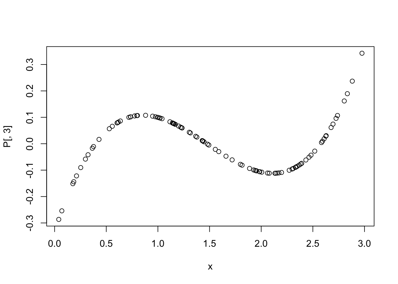
## 109.0490 621.0930 239.6857

To remove multicollinearity in polynomial regression, we can use orthogonal polynomials instead of raw polynomials. This can be done using the poly function in R.

P <- poly(x, 3, raw = FALSE) #orthogonal polynomials
head(P)

##                1           2           3
## [1,] -0.09477731 -0.01967963  0.10653921
## [2,] -0.05473305 -0.08090358  0.08306444
## [3,]  0.02066015 -0.10185681 -0.06116614
## [4,]  0.14661795  0.13798027  0.09603581
## [5,] -0.11875038  0.03360430  0.07885130
## [6,]  0.14293031  0.12607236  0.07431485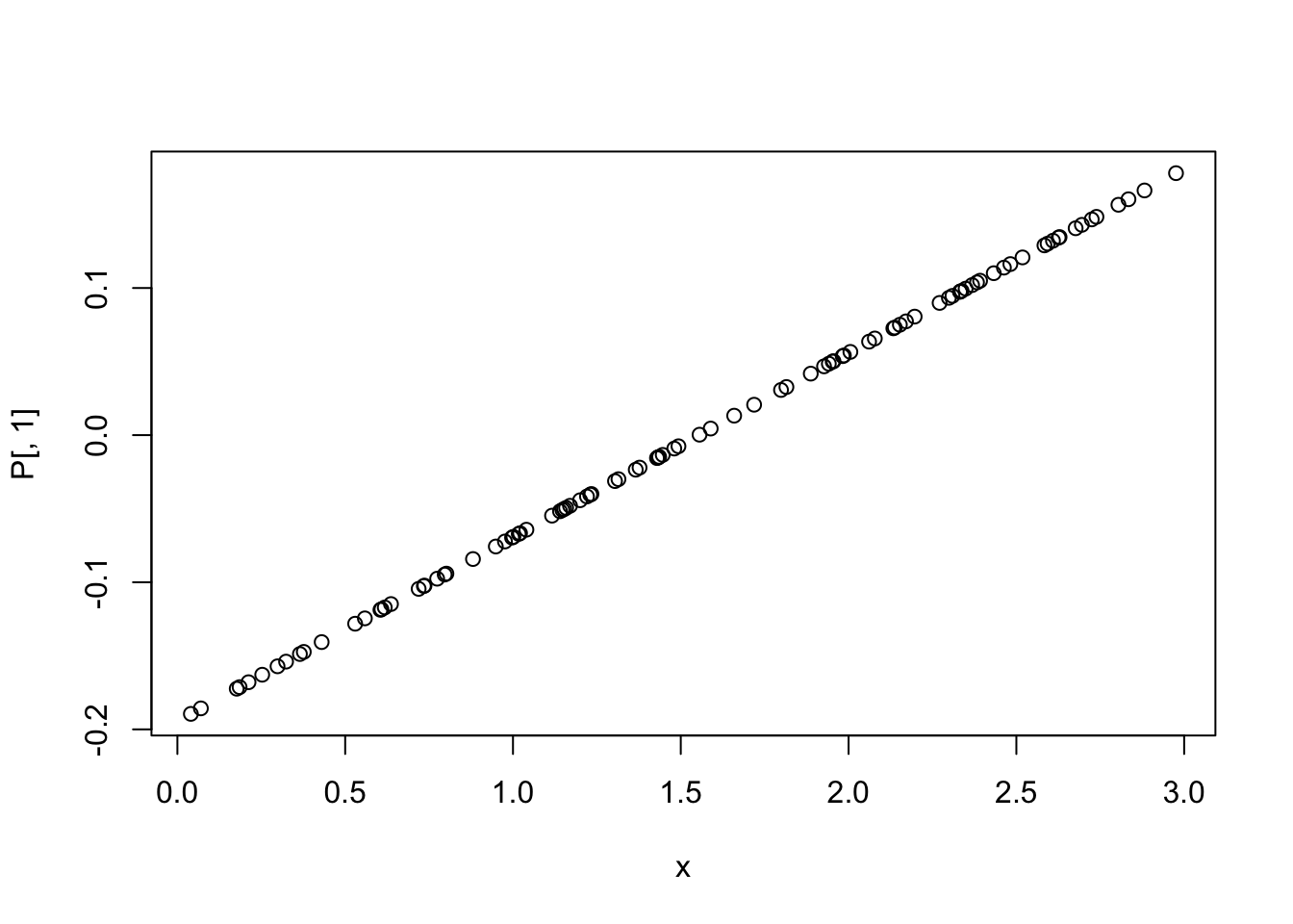

plot(x,P[,1]) #first orthogonal polynomial

plot(x, P[,2]) #second orthogonal polynomial

plot(x, P[,3]) #third orthogonal polynomial

P <- data.frame(P,check.names = T)
P$y <- y
mod2 <- lm(y ~ ., data = P) #using orthogonal polynomials
summary(mod2)

## 
## Call:
## lm(formula = y ~ ., data = P)
## 
## Residuals:
##      Min       1Q   Median       3Q      Max 
## -1.85466 -0.59246 -0.09722  0.54144  2.48360 
## 
## Coefficients:
##             Estimate Std. Error t value Pr(>|t|)    
## (Intercept)  4.79096    0.09496  50.451  < 2e-16 ***
## X1          20.11185    0.94962  21.179  < 2e-16 ***
## X2           4.78141    0.94962   5.035 2.23e-06 ***
## X3           1.80602    0.94962   1.902   0.0602 .  
## ---
## Signif. codes:  0 '***' 0.001 '**' 0.01 '*' 0.05 '.' 0.1 ' ' 1
## 
## Residual standard error: 0.9496 on 96 degrees of freedom
## Multiple R-squared:  0.8326, Adjusted R-squared:  0.8274 
## F-statistic: 159.2 on 3 and 96 DF,  p-value: < 2.2e-16

car::vif(mod2) #no multicollinearity here

## X1 X2 X3 
##  1  1  1

For model selection, it is generally better to use orthogonal polynomials when including polynomial terms in a regression model, because they do not suffer from multicollinearity. That means it is easier to determine whether to remove the cubic predictor, for example, based on its p-value.

10.4 February 10

10.4.1 ANOVA Models

ANOVA (Analysis of Variance) models are a special case of linear regression models where the predictors are categorical variables (factors). They are used to compare the means of different groups and to determine if there are significant differences between them. We have already studied linear models which contain only categorical data, so this is a review of that material with some additional nuances.

We begin with a brief review of one-way ANOVA models, which contain a single categorical predictor. The model can be written as \[ y_{ij} = \mu + \alpha_i + \epsilon_{ij} \] where \(y_{ij}\) is the response variable for the \(j\)th observation in group \(i\), \(\mu\) is the overall mean, \(\alpha_i\) is the effect of group \(i\), and \(\epsilon_{ij}\) is the random error term. The null hypothesis is that all group means are equal, i.e., \(\alpha_1 = \alpha_2 = \ldots = \alpha_k = 0\). This way of writing the model is called the effects coding. Another way to write the model is the treatment coding, which is more common in R, and is given by \[ y_{ij} = \beta_0 + \beta_i D_i + \epsilon_{ij} \] where \(D_i\) is a dummy variable that is 1 if the observation is in group \(i\) and 0 otherwise. In this case, \(\beta_0\) is the mean of the reference group (usually the first group), and \(\beta_i\) is the difference between the mean of group \(i\) and the mean of the reference group.

We assume that the errors are normally distributed with mean 0 and constant variance. The ANOVA table partitions the total variability in the data into variability between groups and variability within groups. The F-statistic is used to test the null hypothesis, and is computed as the ratio of the mean square between groups to the mean square within groups.

Let’s look at an example using the penguins data set to compare body mass across species.

library(ggplot2)
penguins |>
  ggplot(aes(x = species, y = body_mass)) + 
  geom_boxplot() + 
  labs(title = "Body Mass by Penguin Species",
       x = "Species",
       y = "Body Mass (g)") #approximately normal with equal variances

## Warning: Removed 2 rows containing non-finite outside the scale range
## (`stat_boxplot()`).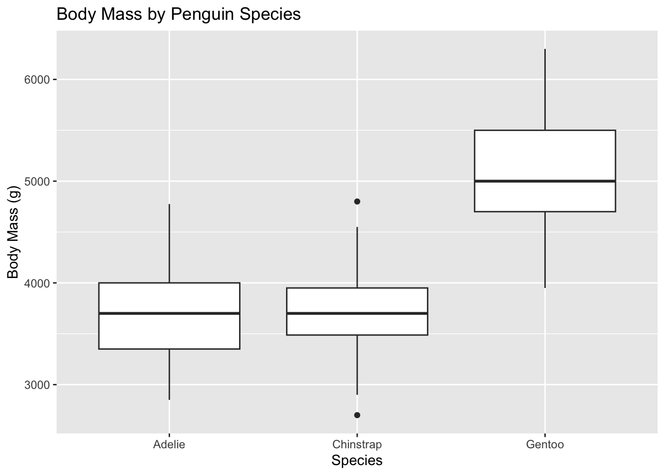

mod <- lm(body_mass ~ species, data = penguins)
summary(mod)

## 
## Call:
## lm(formula = body_mass ~ species, data = penguins)
## 
## Residuals:
##      Min       1Q   Median       3Q      Max 
## -1126.02  -333.09   -33.09   316.91  1223.98 
## 
## Coefficients:
##                  Estimate Std. Error t value Pr(>|t|)    
## (Intercept)       3700.66      37.62   98.37   <2e-16 ***
## speciesChinstrap    32.43      67.51    0.48    0.631    
## speciesGentoo     1375.35      56.15   24.50   <2e-16 ***
## ---
## Signif. codes:  0 '***' 0.001 '**' 0.01 '*' 0.05 '.' 0.1 ' ' 1
## 
## Residual standard error: 462.3 on 339 degrees of freedom
##   (2 observations deleted due to missingness)
## Multiple R-squared:  0.6697, Adjusted R-squared:  0.6677 
## F-statistic: 343.6 on 2 and 339 DF,  p-value: < 2.2e-16

anova(mod)

## Analysis of Variance Table
## 
## Response: body_mass
##            Df    Sum Sq  Mean Sq F value    Pr(>F)    
## species     2 146864214 73432107  343.63 < 2.2e-16 ***
## Residuals 339  72443483   213698                      
## ---
## Signif. codes:  0 '***' 0.001 '**' 0.01 '*' 0.05 '.' 0.1 ' ' 1

Note that the p-value from the ANOVA table matches the p-value for the overall F-test in the linear model summary. If we wish to determine which species are different from each other, we can use post-hoc tests such as Tukey’s HSD.

library(emmeans)

## Welcome to emmeans.
## Caution: You lose important information if you filter this package's results.
## See '? untidy'

emmeans_mod <- emmeans(mod, ~ species)
pairs(emmeans_mod)

##  contrast           estimate   SE  df t.ratio p.value
##  Adelie - Chinstrap    -32.4 67.5 339  -0.480  0.8807
##  Adelie - Gentoo     -1375.4 56.1 339 -24.495  <.0001
##  Chinstrap - Gentoo  -1342.9 69.9 339 -19.224  <.0001
## 
## P value adjustment: tukey method for comparing a family of 3 estimates

Now let’s look at two-way ANOVA models, which contain two categorical predictors. The model can be written as

\[ y_{ijk} = \mu + \alpha_i + \beta_j + (\alpha\beta)_{ij} + \epsilon_{ijk} \] where \(y_{ijk}\) is the response variable for the \(k\)th observation in group \(i\) of factor A and group \(j\) of factor B, \(\mu\) is the overall mean, \(\alpha_i\) is the effect of level \(i\) of factor A, \(\beta_j\) is the effect of level \(j\) of factor B, \((\alpha\beta)_{ij}\) is the interaction effect between levels \(i\) and \(j\), and \(\epsilon_{ijk}\) is the random error term. The null hypotheses are that all main effects and interaction effects are equal to zero.

Let’s look at an example using the ToothGrowth data set, which contains data on tooth length in guinea pigs under different doses of vitamin C and different delivery methods (orange juice vs. ascorbic acid).

data("ToothGrowth")
head(ToothGrowth)

##    len supp dose
## 1  4.2   VC  0.5
## 2 11.5   VC  0.5
## 3  7.3   VC  0.5
## 4  5.8   VC  0.5
## 5  6.4   VC  0.5
## 6 10.0   VC  0.5

tt <- ToothGrowth |>
  mutate(dose = factor(dose)) 
ggplot(tt, aes(x = dose, y = len, fill = supp)) +
  geom_boxplot(position = position_dodge(0.8)) + 
  labs(title = "Tooth Length by Dose and Supplement Type",
       x = "Dose (mg)",
       y = "Tooth Length (mm)")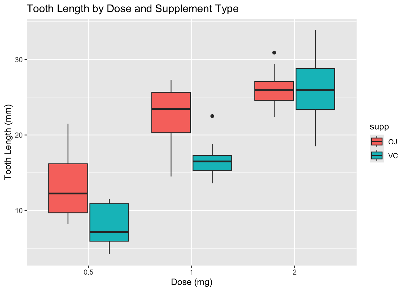

Note that the boxplots suggest a potential interaction between dose and supplement type. It also looks like the variances are not equal across groups, especially at higher doses. Let’s examine the variances more closely.

tt |> 
  group_by(dose, supp) |> 
  summarize(var_len = sd(len), n = n())

## `summarise()` has grouped output by 'dose'. You can override using the
## `.groups` argument.

## # A tibble: 6 × 4
## # Groups:   dose [3]
##   dose  supp  var_len     n
##   <fct> <fct>   <dbl> <int>
## 1 0.5   OJ       4.46    10
## 2 0.5   VC       2.75    10
## 3 1     OJ       3.91    10
## 4 1     VC       2.52    10
## 5 2     OJ       2.66    10
## 6 2     VC       4.80    10

There is some variation in the standard deviations across groups, but it is not extreme. Also note that the study is balanced, with equal sample sizes in each group, which helps mitigate the impact of unequal variances.

Let’s fit the two-way ANOVA model with interaction.

mod2 <- lm(len ~ dose * supp, data = tt)
summary(mod2)

## 
## Call:
## lm(formula = len ~ dose * supp, data = tt)
## 
## Residuals:
##    Min     1Q Median     3Q    Max 
##  -8.20  -2.72  -0.27   2.65   8.27 
## 
## Coefficients:
##              Estimate Std. Error t value Pr(>|t|)    
## (Intercept)    13.230      1.148  11.521 3.60e-16 ***
## dose1           9.470      1.624   5.831 3.18e-07 ***
## dose2          12.830      1.624   7.900 1.43e-10 ***
## suppVC         -5.250      1.624  -3.233  0.00209 ** 
## dose1:suppVC   -0.680      2.297  -0.296  0.76831    
## dose2:suppVC    5.330      2.297   2.321  0.02411 *  
## ---
## Signif. codes:  0 '***' 0.001 '**' 0.01 '*' 0.05 '.' 0.1 ' ' 1
## 
## Residual standard error: 3.631 on 54 degrees of freedom
## Multiple R-squared:  0.7937, Adjusted R-squared:  0.7746 
## F-statistic: 41.56 on 5 and 54 DF,  p-value: < 2.2e-16

anova(mod2)

## Analysis of Variance Table
## 
## Response: len
##           Df  Sum Sq Mean Sq F value    Pr(>F)    
## dose       2 2426.43 1213.22  92.000 < 2.2e-16 ***
## supp       1  205.35  205.35  15.572 0.0002312 ***
## dose:supp  2  108.32   54.16   4.107 0.0218603 *  
## Residuals 54  712.11   13.19                      
## ---
## Signif. codes:  0 '***' 0.001 '**' 0.01 '*' 0.05 '.' 0.1 ' ' 1

To interpret the ANOVA table, we note that the p-value for the interaction term tests whether the effect of dose on tooth length depends on the type of supplement. If the interaction is significant, we should be cautious in interpreting the main effects, as they may not represent the overall effects across all levels of the other factor. If the interaction is not significant, we can consider removing it from the model and interpreting the main effects directly. Let’s check the interaction plot to visualize the interaction effect.

ggplot(tt, aes(x = dose, y = len, color = supp, group = supp)) +
  geom_point(position = position_dodge(0.2)) +
  geom_line(position = position_dodge(0.2)) +
  labs(title = "Interaction Plot: Tooth Length by Dose and Supplement Type",
       x = "Dose (mg)",
       y = "Tooth Length (mm)")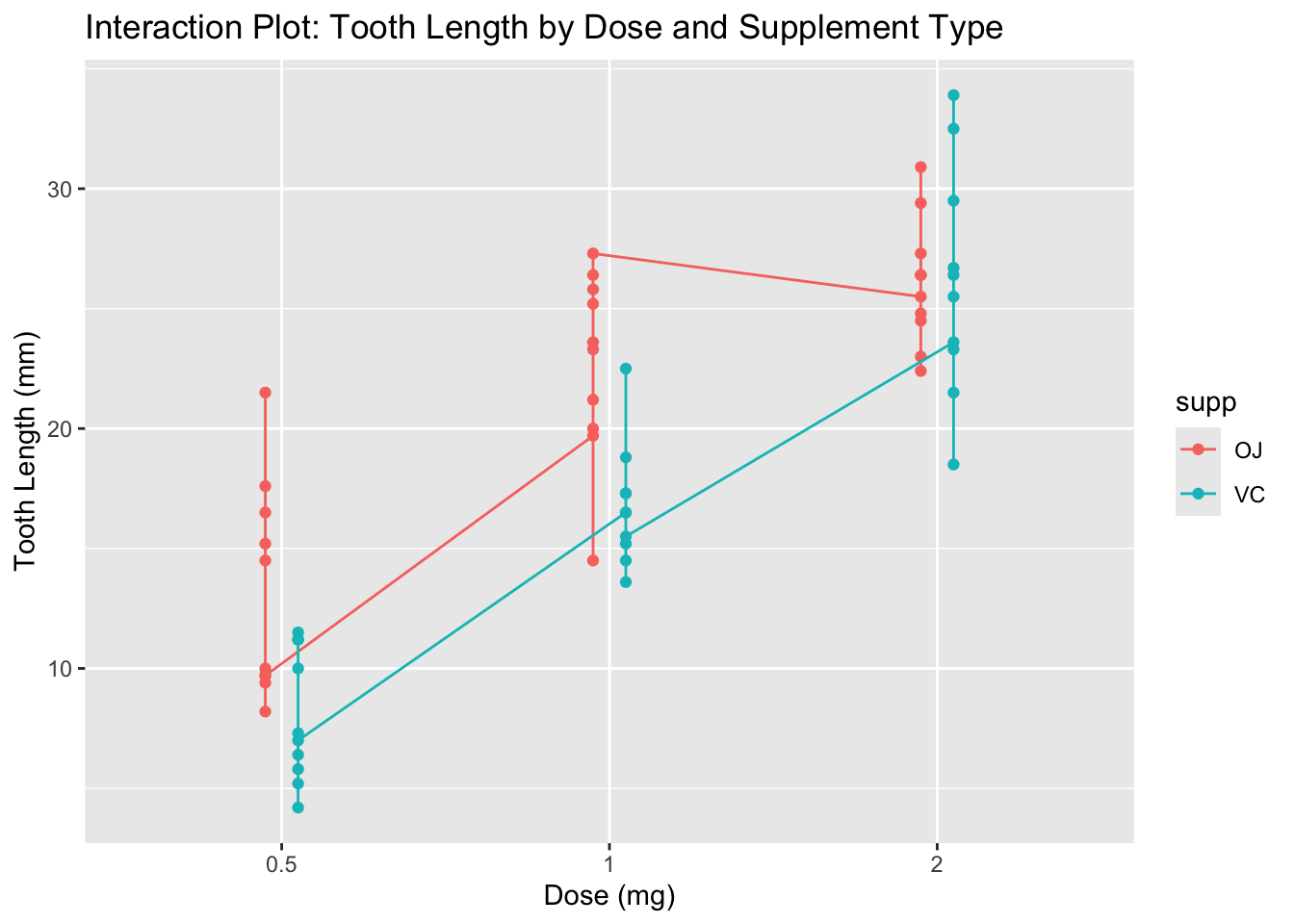

It appears that OJ at doses 0.5 and 1.0 results in longer tooth lengths compared to VC, but at dose 2.0, both supplements yield similar tooth lengths. This suggests a potential interaction effect.

If we decide to remove the interaction term, we can refit the model without it and interpret the main effects.

mod3 <- lm(len ~ dose + supp, data = tt)
summary(mod3)

## 
## Call:
## lm(formula = len ~ dose + supp, data = tt)
## 
## Residuals:
##    Min     1Q Median     3Q    Max 
## -7.085 -2.751 -0.800  2.446  9.650 
## 
## Coefficients:
##             Estimate Std. Error t value Pr(>|t|)    
## (Intercept)  12.4550     0.9883  12.603  < 2e-16 ***
## dose1         9.1300     1.2104   7.543 4.38e-10 ***
## dose2        15.4950     1.2104  12.802  < 2e-16 ***
## suppVC       -3.7000     0.9883  -3.744 0.000429 ***
## ---
## Signif. codes:  0 '***' 0.001 '**' 0.01 '*' 0.05 '.' 0.1 ' ' 1
## 
## Residual standard error: 3.828 on 56 degrees of freedom
## Multiple R-squared:  0.7623, Adjusted R-squared:  0.7496 
## F-statistic: 59.88 on 3 and 56 DF,  p-value: < 2.2e-16

anova(mod3)

## Analysis of Variance Table
## 
## Response: len
##           Df  Sum Sq Mean Sq F value    Pr(>F)    
## dose       2 2426.43 1213.22  82.811 < 2.2e-16 ***
## supp       1  205.35  205.35  14.017 0.0004293 ***
## Residuals 56  820.43   14.65                      
## ---
## Signif. codes:  0 '***' 0.001 '**' 0.01 '*' 0.05 '.' 0.1 ' ' 1

However, in this case, the interaction term was significant, so we should keep it in the model and interpret the effects accordingly.

emmeans_mod2 <- emmeans(mod2, ~ dose * supp)
pairs(emmeans_mod2)

##  contrast                estimate   SE df t.ratio p.value
##  dose0.5 OJ - dose1 OJ      -9.47 1.62 54  -5.831  <.0001
##  dose0.5 OJ - dose2 OJ     -12.83 1.62 54  -7.900  <.0001
##  dose0.5 OJ - dose0.5 VC     5.25 1.62 54   3.233  0.0243
##  dose0.5 OJ - dose1 VC      -3.54 1.62 54  -2.180  0.2640
##  dose0.5 OJ - dose2 VC     -12.91 1.62 54  -7.949  <.0001
##  dose1 OJ - dose2 OJ        -3.36 1.62 54  -2.069  0.3187
##  dose1 OJ - dose0.5 VC      14.72 1.62 54   9.064  <.0001
##  dose1 OJ - dose1 VC         5.93 1.62 54   3.651  0.0074
##  dose1 OJ - dose2 VC        -3.44 1.62 54  -2.118  0.2936
##  dose2 OJ - dose0.5 VC      18.08 1.62 54  11.133  <.0001
##  dose2 OJ - dose1 VC         9.29 1.62 54   5.720  <.0001
##  dose2 OJ - dose2 VC        -0.08 1.62 54  -0.049  1.0000
##  dose0.5 VC - dose1 VC      -8.79 1.62 54  -5.413  <.0001
##  dose0.5 VC - dose2 VC     -18.16 1.62 54 -11.182  <.0001
##  dose1 VC - dose2 VC        -9.37 1.62 54  -5.770  <.0001
## 
## P value adjustment: tukey method for comparing a family of 6 estimates

This provides tests of all pairs of possible interactions. It can be hard to interpret so much output, and we also need to be careful about multiple comparisons. Let’s suppose that our research question is: “how do the dose level effects differ by supplement type?” We can use emmeans to answer this specific question.

emm <- emmeans(mod2, ~ dose | supp)
pairs(emm)

## supp = OJ:
##  contrast        estimate   SE df t.ratio p.value
##  dose0.5 - dose1    -9.47 1.62 54  -5.831  <.0001
##  dose0.5 - dose2   -12.83 1.62 54  -7.900  <.0001
##  dose1 - dose2      -3.36 1.62 54  -2.069  0.1060
## 
## supp = VC:
##  contrast        estimate   SE df t.ratio p.value
##  dose0.5 - dose1    -8.79 1.62 54  -5.413  <.0001
##  dose0.5 - dose2   -18.16 1.62 54 -11.182  <.0001
##  dose1 - dose2      -9.37 1.62 54  -5.770  <.0001
## 
## P value adjustment: tukey method for comparing a family of 3 estimates

This indicates that tooth growth increases with dose for both supplement types, but for OJ the increase is not significant from dose 1 to dose 2, while for VC the increase is significant at each step. To improve this, we might only want to test the increase in dosages from 0.5 to 1 and from 1 to 2, because the increase from 0.5 to 2 is redundant. We can do this by specifying contrasts in emmeans.

contrast(emm, method = "trt.vs.ctrl", by = "supp", adjust = "holm")

## supp = OJ:
##  contrast        estimate   SE df t.ratio p.value
##  dose1 - dose0.5     9.47 1.62 54   5.831  <.0001
##  dose2 - dose0.5    12.83 1.62 54   7.900  <.0001
## 
## supp = VC:
##  contrast        estimate   SE df t.ratio p.value
##  dose1 - dose0.5     8.79 1.62 54   5.413  <.0001
##  dose2 - dose0.5    18.16 1.62 54  11.182  <.0001
## 
## P value adjustment: holm method for 2 tests

In this case, we note that contrast chooses the base level of the factor as the control group. So for dose, the control is 0.5, and we are testing 1 vs 0.5 and 2 vs 0.5. The Holm adjustment is a way to control the family-wise error rate when making multiple comparisons. If we wanted to test 0.5 vs 1 and 1 vs 2 instead, we would need to reorder the levels of the factor dose so that 1 is the base level. This is not really treatment vs control, but the function is flexible enough to handle this situation.

10.4.2 Heading towards mixed models

Now, we return to linear models with interactions. We imagine a scenario where we have several (perhaps more than several) groups of data, and we have a few observations in each group. Let’s consider the sleepstudy data set in the lme4 package.

library(lme4)

## Loading required package: Matrix

## 
## Attaching package: 'Matrix'

## The following objects are masked from 'package:tidyr':
## 
##     expand, pack, unpack

data("sleepstudy")
ss <- sleepstudy |> 
  janitor::clean_names()
summary(ss)

##     reaction          days        subject   
##  Min.   :194.3   Min.   :0.0   308    : 10  
##  1st Qu.:255.4   1st Qu.:2.0   309    : 10  
##  Median :288.7   Median :4.5   310    : 10  
##  Mean   :298.5   Mean   :4.5   330    : 10  
##  3rd Qu.:336.8   3rd Qu.:7.0   331    : 10  
##  Max.   :466.4   Max.   :9.0   332    : 10  
##                                (Other):120

length(unique(ss$subject)) #18 groups, 10 observations per group

## [1] 18

ss |> 
  ggplot(aes(x = days, y = reaction, color = subject)) + 
  geom_point() + 
  geom_smooth(method = "lm", se = F)

## `geom_smooth()` using formula = 'y ~ x'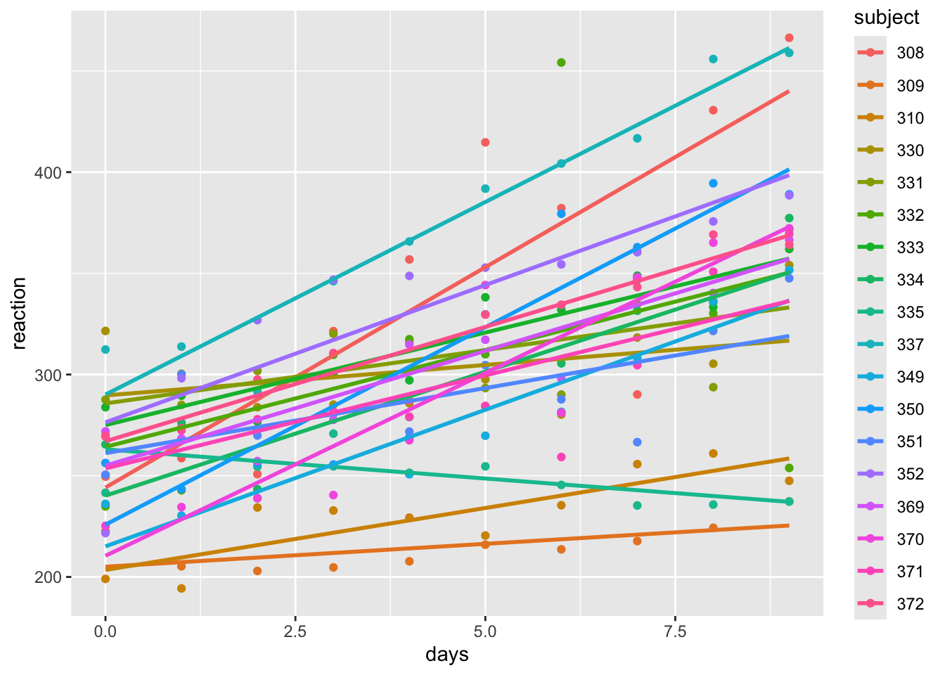

Based on this data, it seems that we have potentially different intercepts and slopes for each subject. Let’s fit a linear model with an interaction between days and subject. We will have 18 intercepts and 18 slopes, which is a lot of parameters to estimate with only 180 observations. (It is five observations per parameter estimated - how much confidence would you have in an estimated mean based off of 5 observations? Mathematically, it is fine. But in practice, it is not ideal.)

mod <- lm(reaction ~ days * subject, data = ss)
summary(mod)

## 
## Call:
## lm(formula = reaction ~ days * subject, data = ss)
## 
## Residuals:
##      Min       1Q   Median       3Q      Max 
## -106.397  -10.692   -0.177   11.417  132.510 
## 
## Coefficients:
##                 Estimate Std. Error t value Pr(>|t|)    
## (Intercept)      244.193     15.042  16.234  < 2e-16 ***
## days              21.765      2.818   7.725 1.74e-12 ***
## subject309       -39.138     21.272  -1.840 0.067848 .  
## subject310       -40.708     21.272  -1.914 0.057643 .  
## subject330        45.492     21.272   2.139 0.034156 *  
## subject331        41.546     21.272   1.953 0.052749 .  
## subject332        20.059     21.272   0.943 0.347277    
## subject333        30.826     21.272   1.449 0.149471    
## subject334        -4.030     21.272  -0.189 0.850016    
## subject335        18.842     21.272   0.886 0.377224    
## subject337        45.911     21.272   2.158 0.032563 *  
## subject349       -29.081     21.272  -1.367 0.173728    
## subject350       -18.358     21.272  -0.863 0.389568    
## subject351        16.954     21.272   0.797 0.426751    
## subject352        32.179     21.272   1.513 0.132535    
## subject369        10.775     21.272   0.507 0.613243    
## subject370       -33.744     21.272  -1.586 0.114870    
## subject371         9.443     21.272   0.444 0.657759    
## subject372        22.852     21.272   1.074 0.284497    
## days:subject309  -19.503      3.985  -4.895 2.61e-06 ***
## days:subject310  -15.650      3.985  -3.928 0.000133 ***
## days:subject330  -18.757      3.985  -4.707 5.84e-06 ***
## days:subject331  -16.499      3.985  -4.141 5.88e-05 ***
## days:subject332  -12.198      3.985  -3.061 0.002630 ** 
## days:subject333  -12.623      3.985  -3.168 0.001876 ** 
## days:subject334   -9.512      3.985  -2.387 0.018282 *  
## days:subject335  -24.646      3.985  -6.185 6.07e-09 ***
## days:subject337   -2.739      3.985  -0.687 0.492986    
## days:subject349   -8.271      3.985  -2.076 0.039704 *  
## days:subject350   -2.261      3.985  -0.567 0.571360    
## days:subject351  -15.331      3.985  -3.848 0.000179 ***
## days:subject352   -8.198      3.985  -2.057 0.041448 *  
## days:subject369  -10.417      3.985  -2.614 0.009895 ** 
## days:subject370   -3.709      3.985  -0.931 0.353560    
## days:subject371  -12.576      3.985  -3.156 0.001947 ** 
## days:subject372  -10.467      3.985  -2.627 0.009554 ** 
## ---
## Signif. codes:  0 '***' 0.001 '**' 0.01 '*' 0.05 '.' 0.1 ' ' 1
## 
## Residual standard error: 25.59 on 144 degrees of freedom
## Multiple R-squared:  0.8339, Adjusted R-squared:  0.7936 
## F-statistic: 20.66 on 35 and 144 DF,  p-value: < 2.2e-16

We can see that it appears that both the intercept and the slope change with the subject. Following what we had done before, we would be done with our modeling. Here are some issues:

We have no way to predict the reaction time for a new subject that is not in our data set, because we have no estimate of the intercept or slope for that subject.
How would we answer the following question: is reaction time associated with number of days of sleep deprivation? We could look at the overall F-test for the model, but that is not really testing the association between reaction time and days of sleep deprivation. It is testing whether there is an association between reaction time and days of sleep deprivation for each subject. We would like to be able to test the overall association between reaction time and days of sleep deprivation, while accounting for the fact that we have different intercepts and slopes for each subject. Based on the plot, it seems like for some subjects, the reaction time might be getting faster with more sleep deprivation.
We have a lot of parameters in this model, which can lead to overfitting. We haven’t really talked much about overfitting in this class yet. But, when we are looking for a parsimonious model by variable selection, we are trying to avoid overfitting. In this case, we have a lot of parameters, and we are not really interested in the individual intercepts and slopes for each subject. We are more interested in the overall association between reaction time and days of sleep deprivation, while accounting for the fact that we have (possibly) different intercepts and slopes for each subject.

What is wrong with forgetting that we have the same subjects, and running the following regression?

#THIS IS NOT ADVISED
mod_wrong <- lm(reaction ~ days, data = ss)
summary(mod_wrong)

## 
## Call:
## lm(formula = reaction ~ days, data = ss)
## 
## Residuals:
##      Min       1Q   Median       3Q      Max 
## -110.848  -27.483    1.546   26.142  139.953 
## 
## Coefficients:
##             Estimate Std. Error t value Pr(>|t|)    
## (Intercept)  251.405      6.610  38.033  < 2e-16 ***
## days          10.467      1.238   8.454 9.89e-15 ***
## ---
## Signif. codes:  0 '***' 0.001 '**' 0.01 '*' 0.05 '.' 0.1 ' ' 1
## 
## Residual standard error: 47.71 on 178 degrees of freedom
## Multiple R-squared:  0.2865, Adjusted R-squared:  0.2825 
## F-statistic: 71.46 on 1 and 178 DF,  p-value: 9.894e-15

This model is not accounting for the fact that we have repeated measurements for each subject. It is treating each observation as independent, which is not the case. This can lead to underestimated standard errors and inflated type I error rates. We need a way to account for the fact that we have repeated measurements for each subject, and that the intercepts and slopes may vary by subject. This is where mixed models come in, which we will cover in the next lecture.

10.4.3 Intro to Random Effects and Mixed Effect Models - Terminology and First Examples

First off, let’s get some terminology down. A fixed effect is an effect that is constant across individuals or groups. For example, the effect of a treatment in a clinical trial is often considered a fixed effect, because we are interested in the average effect of the treatment across all individuals. This is a modeling decision that we make based on our research question and the structure of our data. In the sleepstudy data set, the effect of days on reaction could be considered a fixed effect, because we are interested in the overall association between days of sleep deprivation and reaction time across all subjects.

A random effect is an effect that varies across individuals or groups. For example, the intercepts and slopes for each subject in the sleepstudy data set can be considered random effects, because they vary across subjects. A mixed effect model is a model that contains both fixed effects and random effects. In the sleepstudy data set, a mixed effect model would include the fixed effect of days and the random effects of the intercepts and slopes for each subject.

Mixed effect models go by many different names in different disciplines. If you hear these words, the person may be talking about mixed effect models or something very similar:

multilevel models
hierarchical linear models
random effects models
linear mixed models
Variance components models
BLUP models (genetics)
Penalized least squares (numerical analysis - these are more general than mixed models, but they include mixed models as a special case)
Probably many more

Let’s start by fully specifying a mixed effect model which includes a random intercept and a fixed effect slope of one variable. The model can be written as \[ y_{ij} = \beta_0 + \beta_1 x_{ij} + b_{0i} + \epsilon_{ij} \] where \(y_{ij}\) is the response variable for the \(j\)th observation in group \(i\), \(\beta_0\) is the overall intercept, \(\beta_1\) is the fixed effect slope for predictor \(x\), \(b_{0i}\) is the random intercept for group \(i\), and \(\epsilon_{ij}\) is the random error term. We assume that the random effects \(b_{0i}\) are normally distributed with mean 0 and variance \(\sigma_b^2\), and that the errors \(\epsilon_{ij}\) are normally distributed with mean 0 and variance \(\sigma^2\). The random effects and errors are assumed to be independent of each other.

Note that we are splitting the mean of the intercept and the variance of the intercept into two components. We could also have said the \(b_{0i}\) are normal with mean \(\beta_0\) and variance \(\sigma_b^2\).

The fixed effect \(\beta_1\) represents the average effect of predictor \(x\) on the response variable across all groups, while the random effects \(b_{0i}\) represent the deviation of each group’s intercept from the overall intercept \(\beta_0\). The variance \(\sigma_b^2\) captures the variability in the intercepts across groups, while \(\sigma^2\) captures the variability within groups.

Here is how we can simulate data like this:

g <- 10 #number of groups
n <- 5 # observations per group
groups <- factor(letters[1:g]) #this only works if g <= 26!
set.seed(1)
x <- runif(g * n, 0, 10) #these are the predictors
sigma_b <- 2
b0 <- rnorm(g, 0, sigma_b) #these are the random intercepts for each group
beta0 <- 3
beta1 <- 0.5
sigma <- 1
y <- beta0 + beta1 * x + rep(b0, each = n) + rnorm(g * n, 0, sigma) #these are the responses, note that sigma^2 = 1, beta_0 = 3, and beta_1 = 0.5
dd <- data.frame(x = x,
                 y = y,
                 g = rep(groups, each = n))
ggplot(dd, aes(x = x, y = y, color = g)) + 
  geom_point() + 
  geom_smooth(method = "lm", se = F)

## `geom_smooth()` using formula = 'y ~ x'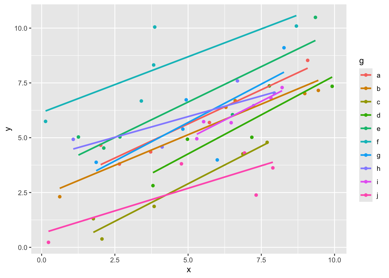

Here we can see that the slopes all look more or less the same, but the intercepts are probably different. Let’s see how we could estimate the parameters in our model. This is not exactly how the programs that we use will do it, but it gives a flavor of the ideas.

First, we could estimate the fixed effect slope \(\beta_1\) and the mean of the random intercept \(\beta_0\) by fitting a linear model that ignores the grouping structure of the data. This is not ideal, but it gives us a starting point. We should definitely not use the \(p\)-values.

mod_fixed <- lm(y ~ x, data = dd)
summary(mod_fixed)

## 
## Call:
## lm(formula = y ~ x, data = dd)
## 
## Residuals:
##     Min      1Q  Median      3Q     Max 
## -4.0639 -1.2257  0.0424  0.8666  5.3072 
## 
## Coefficients:
##             Estimate Std. Error t value Pr(>|t|)    
## (Intercept)  2.84025    0.59583   4.767 1.77e-05 ***
## x            0.49262    0.09982   4.935 1.01e-05 ***
## ---
## Signif. codes:  0 '***' 0.001 '**' 0.01 '*' 0.05 '.' 0.1 ' ' 1
## 
## Residual standard error: 1.902 on 48 degrees of freedom
## Multiple R-squared:  0.3366, Adjusted R-squared:  0.3228 
## F-statistic: 24.35 on 1 and 48 DF,  p-value: 1.005e-05

Next, we could estimate the random effects \(b_{0i}\) by fitting a linear model that includes the group as a fixed effect. This will give us estimates of the intercepts for each group, which we can then use to estimate the variance of the random effects.

mod_full <- lm(y ~ x + g, data = dd)
summary(mod_full)

## 
## Call:
## lm(formula = y ~ x + g, data = dd)
## 
## Residuals:
##     Min      1Q  Median      3Q     Max 
## -2.2982 -0.5209 -0.1299  0.5674  1.9430 
## 
## Coefficients:
##             Estimate Std. Error t value Pr(>|t|)    
## (Intercept)  2.75627    0.49259   5.596 1.89e-06 ***
## x            0.57119    0.05334  10.709 3.55e-13 ***
## gb          -0.49336    0.60947  -0.809   0.4231    
## gc          -2.77550    0.60238  -4.608 4.28e-05 ***
## gd          -1.10549    0.61250  -1.805   0.0788 .  
## ge           0.96834    0.60245   1.607   0.1160    
## gf           3.14483    0.60331   5.213 6.39e-06 ***
## gg           0.10459    0.60297   0.173   0.8632    
## gh           0.27154    0.60369   0.450   0.6553    
## gi          -0.47174    0.61191  -0.771   0.4454    
## gj          -2.98804    0.60376  -4.949 1.47e-05 ***
## ---
## Signif. codes:  0 '***' 0.001 '**' 0.01 '*' 0.05 '.' 0.1 ' ' 1
## 
## Residual standard error: 0.9523 on 39 degrees of freedom
## Multiple R-squared:  0.8649, Adjusted R-squared:  0.8303 
## F-statistic: 24.97 on 10 and 39 DF,  p-value: 6.241e-14

Finally, we could use the estimates from the previous two models to estimate the variance components \(\sigma_b^2\) and \(\sigma^2\). This is typically done using restricted maximum likelihood (REML) or maximum likelihood (ML) estimation, which are more efficient than the method of moments that we are using here.

broom::tidy(mod_full) |>  
  filter(str_detect(term, "g|tercept")) |>  
  mutate(estimate = ifelse(str_detect(term, "Inter"), 0, estimate)) |> 
  summarize(var_b = var(estimate)) #this is an estimate of sigma_b^2ilt

## # A tibble: 1 × 1
##   var_b
##   <dbl>
## 1  3.12

This is an estimate for the variance of the random intercepts, \(\sigma_b^2\). Recall that the true value was 4. Finally, we can estimate \(\sigma^2\) by looking at the residuals from the full model.

var(resid(mod_full))

## [1] 0.7218008

This is an estimate for the variance of the errors, \(\sigma^2\). Recall that the true value was 1. Note that there are definitely issues with doing this, but in this simple case the estimates that we get are not too far off.

To use more sophisticated tools, we use the package lme4.

mod_mixed <- lme4::lmer(y ~ x + (1 | g), data = dd) #the (1|g) indicates that we have a random intercept. The fixed effects are entered just like before
summary(mod_mixed)

## Linear mixed model fit by REML ['lmerMod']
## Formula: y ~ x + (1 | g)
##    Data: dd
## 
## REML criterion at convergence: 166.8
## 
## Scaled residuals: 
##      Min       1Q   Median       3Q      Max 
## -2.38213 -0.51459 -0.04616  0.52749  2.25158 
## 
## Random effects:
##  Groups   Name        Variance Std.Dev.
##  g        (Intercept) 2.9386   1.7142  
##  Residual             0.9069   0.9523  
## Number of obs: 50, groups:  g, 10
## 
## Fixed effects:
##             Estimate Std. Error t value
## (Intercept)  2.44928    0.62613   3.912
## x            0.56603    0.05312  10.655
## 
## Correlation of Fixed Effects:
##   (Intr)
## x -0.452

This model includes a random intercept for each group, but assumes that the slope is the same across groups. The output gives us estimates for the fixed effects (the overall intercept and slope) as well as the variance components (the variance of the random intercepts and the variance of the errors).